Ripser demonstration¶

This notebook shows the most basic use of the Ripser Python API.

[1]:

%load_ext autoreload
%autoreload 2

[2]:

from ripser import ripser
from persim import plot_diagrams
import matplotlib.pyplot as plt
import numpy as np
from sklearn import datasets

[3]:

data = datasets.make_circles(n_samples=100)[0] + 5 * datasets.make_circles(n_samples=100)[0]

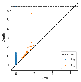
Default args make it very easy.¶

Generate diagrams for \(H_0\) and \(H_1\)
Plot both diagrams

[4]:

dgms = ripser(data)['dgms']
plot_diagrams(dgms, show=True)

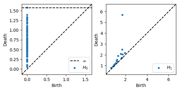
../_images/notebooks_Basic_Usage_5_0.png

[5]:

# Plot each diagram by itself
plot_diagrams(dgms, plot_only=[0], ax=plt.subplot(121))
plot_diagrams(dgms, plot_only=[1], ax=plt.subplot(122))

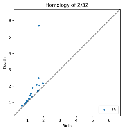
../_images/notebooks_Basic_Usage_6_0.png

Homology over any prime basis¶

We can compute homology over any \(p\ge 2\) by supplying the argument coeff=p.

[6]:

# Homology over Z/3Z
dgms = ripser(data, coeff=3)['dgms']
plot_diagrams(dgms, plot_only=[1], title="Homology of Z/3Z", show=True)

../_images/notebooks_Basic_Usage_8_0.png

[7]:

# Homology over Z/7Z
dgms = ripser(data, coeff=3)['dgms']
plot_diagrams(dgms, plot_only=[1], title="Homology of Z/7Z", show=True) # Only plot H_1

../_images/notebooks_Basic_Usage_9_0.png

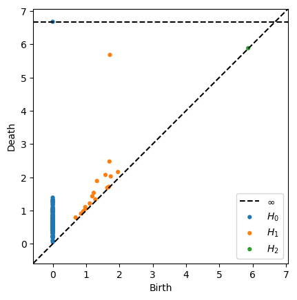
Specify which homology classes to compute¶

We can compute any order of homology, \(H_0, H_1, H_2, \ldots\). By default, we only compute \(H_0\) and \(H_1\). You can specify a larger by supplying the argument maxdim=p. It practice, anything above \(H_1\) is very slow.

[8]:

dgms = ripser(data, maxdim=2)['dgms']
plot_diagrams(dgms, show=True)

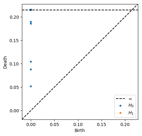
../_images/notebooks_Basic_Usage_11_0.png

Specify maximum radius for Rips filtration¶

We can restrict the maximum radius of the VR complex by supplying the argument thresh=r. Certain classes will not be born if their birth time is under the threshold, and other classes will have infinite death times if their ordinary death time is above the threshold

[9]:

dgms = ripser(data, thresh=0.2)['dgms']
plot_diagrams(dgms, show=True)

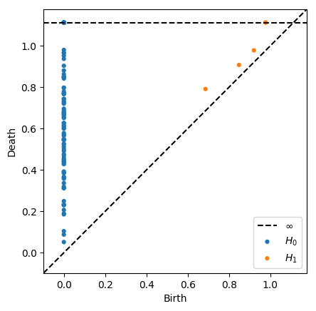
../_images/notebooks_Basic_Usage_13_0.png

[10]:

dgms = ripser(data, thresh=1)['dgms']
plot_diagrams(dgms, show=True)

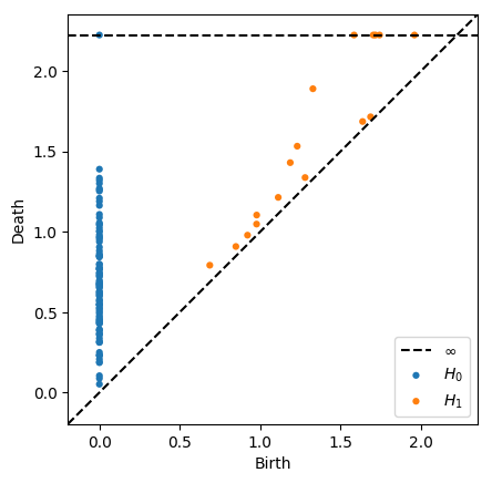
../_images/notebooks_Basic_Usage_14_0.png

[11]:

dgms = ripser(data, thresh=2)['dgms']
plot_diagrams(dgms, show=True)

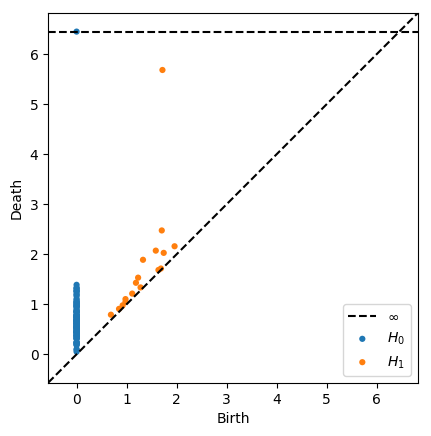
../_images/notebooks_Basic_Usage_15_0.png

[12]:

dgms = ripser(data, thresh=999)['dgms']
plot_diagrams(dgms, show=True)

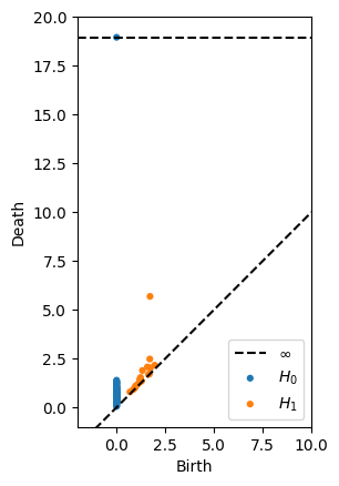
../_images/notebooks_Basic_Usage_16_0.png

Plotting Options¶

[13]:

# This looks weird, but it's possible
plot_diagrams(dgms, xy_range=[-2,10,-1,20])

../_images/notebooks_Basic_Usage_18_0.png

Colormaps¶

See all available color maps with

import matplotlib as mpl
print(mpl.styles.available)

[14]:

plot_diagrams(dgms, colormap='seaborn')

../_images/notebooks_Basic_Usage_20_0.png

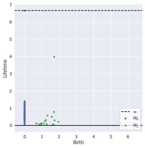
Plot lifetime of generators¶

[15]:

plot_diagrams(dgms, lifetime=True)

../_images/notebooks_Basic_Usage_22_0.png

[ ]: