Approximate Sparse Filtrations

In this module, we will explore an approximation algorithm which is meant to reduce the run time of the persistence algorithm [1]. For more information on this algorithm, please view the following video:

https://www.youtube.com/watch?v=3WxuSwQhAgU

[1] Cavanna, Nicholas J., Mahmoodreza Jahanseir, and Donald R. Sheehy. “A geometric perspective on sparse filtrations.” Proceedings of the Canadian Conference on Computational Geometry (CCCG 2015).

from ripser import ripser
from persim import plot_diagrams
import tadasets

import numpy as np
import matplotlib.pyplot as plt
from sklearn.metrics.pairwise import pairwise_distances
from scipy import sparse
import time

Now, we define a “greedy permutation,” as a function which performs furthest points sampling, a key step in the algorithm used to determine “insertion radii” \(\lambda_i\) for each point. For an animation of how this works, please visit:

https://gist.github.com/ctralie/128cc07da67f1d2e10ea470ee2d23fe8

def getGreedyPerm(D):
    """
    A Naive O(N^2) algorithm to do furthest points sampling

    Parameters
    ----------
    D : ndarray (N, N)
        An NxN distance matrix for points

    Return
    ------
    lamdas: list
        Insertion radii of all points
    """

    N = D.shape[0]
    #By default, takes the first point in the permutation to be the
    #first point in the point cloud, but could be random
    perm = np.zeros(N, dtype=np.int64)
    lambdas = np.zeros(N)
    ds = D[0, :]
    for i in range(1, N):
        idx = np.argmax(ds)
        perm[i] = idx
        lambdas[i] = ds[idx]
        ds = np.minimum(ds, D[idx, :])
    return lambdas[perm]

Now, we define a function which, given a distance matrix representing a point cloud, a set of insertion radii, and an approximation factor \(\epsilon\), returns a sparse distance matrix with re-weighted edges, whose persistence diagrams are each guaranteed to be a \((1+\epsilon)\) multiplicative approximation of the true persistence diagrams (see [1])

def getApproxSparseDM(lambdas, eps, D):
    """
    Purpose: To return the sparse edge list with the warped distances, sorted by weight

    Parameters
    ----------
    lambdas: list
        insertion radii for points
    eps: float
        epsilon approximation constant
    D: ndarray
        NxN distance matrix, okay to modify because last time it's used

    Return
    ------
    DSparse: scipy.sparse
        A sparse NxN matrix with the reweighted edges
    """
    N = D.shape[0]
    E0 = (1+eps)/eps
    E1 = (1+eps)**2/eps

    # Create initial sparse list candidates (Lemma 6)
    # Search neighborhoods
    nBounds = ((eps**2+3*eps+2)/eps)*lambdas

    # Set all distances outside of search neighborhood to infinity
    D[D > nBounds[:, None]] = np.inf
    [I, J] = np.meshgrid(np.arange(N), np.arange(N))
    idx = I < J
    I = I[(D < np.inf)*(idx == 1)]
    J = J[(D < np.inf)*(idx == 1)]
    D = D[(D < np.inf)*(idx == 1)]

    #Prune sparse list and update warped edge lengths (Algorithm 3 pg. 14)
    minlam = np.minimum(lambdas[I], lambdas[J])
    maxlam = np.maximum(lambdas[I], lambdas[J])

    # Rule out edges between vertices whose balls stop growing before they touch
    # or where one of them would have been deleted.  M stores which of these
    # happens first
    M = np.minimum((E0 + E1)*minlam, E0*(minlam + maxlam))

    t = np.arange(len(I))
    t = t[D <= M]
    (I, J, D) = (I[t], J[t], D[t])
    minlam = minlam[t]
    maxlam = maxlam[t]

    # Now figure out the metric of the edges that are actually added
    t = np.ones(len(I))

    # If cones haven't turned into cylinders, metric is unchanged
    t[D <= 2*minlam*E0] = 0

    # Otherwise, if they meet before the M condition above, the metric is warped
    D[t == 1] = 2.0*(D[t == 1] - minlam[t == 1]*E0) # Multiply by 2 convention
    return sparse.coo_matrix((D, (I, J)), shape=(N, N)).tocsr()

Now let’s set up a point cloud we can test this on, which has enough points for ripser to start slowing down a bit. We’ll perform the full rips filtration on this point cloud as a ground truth, and we will time it

X = tadasets.infty_sign(n=2000, noise=0.1)
plt.scatter(X[:, 0], X[:, 1])

tic = time.time()
resultfull = ripser(X)
toc = time.time()
timefull = toc-tic
print("Elapsed Time: %.3g seconds, %i Edges added"%(timefull, resultfull['num_edges']))

Elapsed Time: 19.2 seconds, 1999000 Edges added

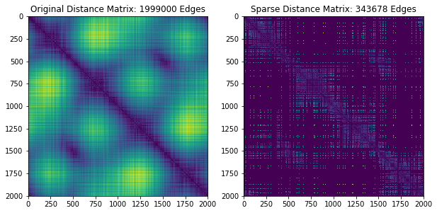
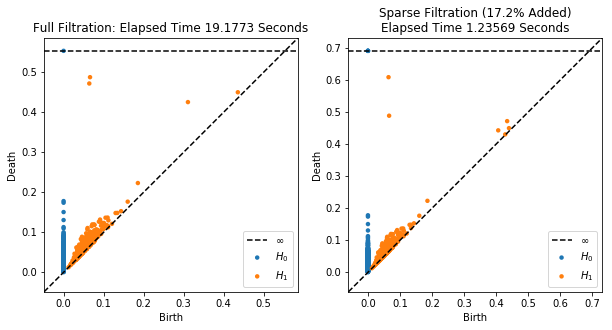
Now let’s run an approximate version and plot \(H_1\) for both next to each other

eps = 0.1

# Compute the sparse filtration
tic = time.time()

# First compute all pairwise distances and do furthest point sampling
D = pairwise_distances(X, metric='euclidean')
lambdas = getGreedyPerm(D)

# Now compute the sparse distance matrix
DSparse = getApproxSparseDM(lambdas, eps, D)

# Finally, compute the filtration
resultsparse = ripser(DSparse, distance_matrix=True)
toc = time.time()
timesparse = toc-tic
percent_added = 100.0*float(resultsparse['num_edges'])/resultfull['num_edges']
print("Elapsed Time: %.3g seconds, %i Edges added"%(timesparse, resultsparse['num_edges']))

Elapsed Time: 1.24 seconds, 343678 Edges added

# Plot the sparse distance matrix and edges that were added
plt.figure(figsize=(10, 5))
plt.subplot(121)
D = pairwise_distances(X, metric='euclidean')
plt.imshow(D)
plt.title("Original Distance Matrix: %i Edges"%resultfull['num_edges'])
plt.subplot(122)
DSparse = DSparse.toarray()
DSparse = DSparse + DSparse.T
plt.imshow(DSparse)
plt.title("Sparse Distance Matrix: %i Edges"%resultsparse['num_edges'])

# And plot the persistence diagrams on top of each other
plt.figure(figsize=(10, 5))
plt.subplot(121)
plot_diagrams(resultfull['dgms'], show=False)
plt.title("Full Filtration: Elapsed Time %g Seconds"%timefull)
plt.subplot(122)
plt.title("Sparse Filtration (%.3g%% Added)\nElapsed Time %g Seconds"%(percent_added, timesparse))
plot_diagrams(resultsparse['dgms'], show=False)

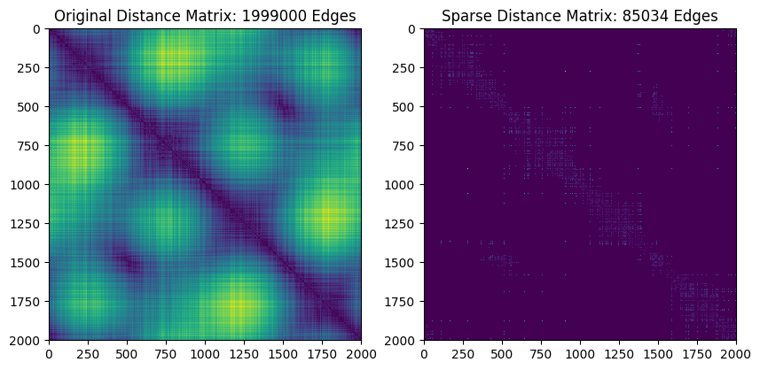
Now we’ll do the exact same thing, but this time we’ll raise epsilon to get a faster, slightly worse approximation

eps = 0.4

# Compute the sparse filtration
tic = time.time()

# First compute all pairwise distances and do furthest point sampling
D = pairwise_distances(X, metric='euclidean')
lambdas = getGreedyPerm(D)

# Now compute the sparse distance matrix
DSparse = getApproxSparseDM(lambdas, eps, D)

# Finally, compute the filtration
resultsparse = ripser(DSparse, distance_matrix=True)
toc = time.time()
timesparse = toc-tic
percent_added = 100.0*float(resultsparse['num_edges'])/resultfull['num_edges']
print("Elapsed Time: %.3g seconds, %i Edges added"%(timesparse, resultsparse['num_edges']))

Elapsed Time: 0.322 seconds, 85034 Edges added

#Plot the sparse distance matrix and edges that were added
plt.figure(figsize=(10, 5))
plt.subplot(121)
D = pairwise_distances(X, metric='euclidean')
plt.imshow(D)
plt.title("Original Distance Matrix: %i Edges"%resultfull['num_edges'])
plt.subplot(122)
DSparse = DSparse.toarray()
DSparse = DSparse + DSparse.T
plt.imshow(DSparse)
plt.title("Sparse Distance Matrix: %i Edges"%resultsparse['num_edges'])

#And plot the persistence diagrams on top of each other
plt.figure(figsize=(10, 5))
plt.subplot(121)
plot_diagrams(resultfull['dgms'], show=False)
plt.title("Full Filtration: Elapsed Time %g Seconds"%timefull)
plt.subplot(122)
plt.title("Sparse Filtration (%.3g%% Added)\nElapsed Time %g Seconds"%(percent_added, timesparse))
plot_diagrams(resultsparse['dgms'], show=False)

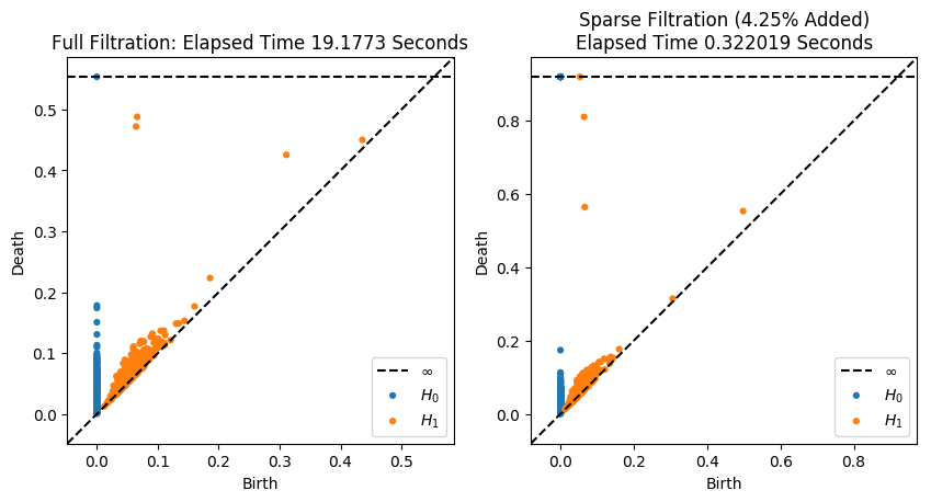
Not bad for nearly two orders of magnitude faster! Mainly, the death times just got a little bit later for the two most important classes in \(H_1\)